Editor’s note: This post was originally published June 6th, 2025.
What is a location-allocation problem in GIS?
Summer’s almost here, so let’s start with a sunny example. Imagine you’re tasked with finding the top 1,000 most profitable locations across the UK to park an ice cream cart. It’s not just about sweet treats, it’s a geospatial location-allocation problem, one that uses data and analysis to determine optimal placement based on demand, foot traffic, and competition.
But let’s be honest: this isn’t really about ice cream carts.
In our personal lives, we constantly solve these kinds of problems, sometimes without even realizing it.
Take a simple scenario: you’re planning a weekly dinner with your five closest friends, each living in different parts of the city. You want to choose a restaurant that minimizes the total travel time for everyone. Or think bigger: you’re looking for a house to rent or buy. You want a location that balances multiple factors: your commute, your partner’s job, your child’s school, your gym, and maybe even your favorite grocery store.
These are location-allocation problems, and they are everywhere.
Governments and businesses face them every day. Where should we place new fire stations to achieve 8-minute response times across a city? Where is the best spot for a new wastewater treatment plant? How do we select optimal locations for bus depots, EV charging stations, or substations to relieve electricity grid congestion?
The list of applications is endless. And the process doesn’t stop after choosing the top candidate locations. You’ll often want to monitor how these locations perform over time. Do they still serve the demand well? Has the population shifted? What insights can we gain from usage data, customer behavior, or operational costs?
This evolution naturally leads into the world of data products, big data, predictive modeling, and machine learning. Since these challenges are inherently spatial, Geographic Information Systems (GIS) remain indispensable, not just for mapping, but as comprehensive information systems that integrate people, data, analysis, software, and hardware. To truly harness the power of GIS and spatial intelligence, you need a platform that supports all these components in a seamless and scalable way.
There are many tools out there to solve these problems, but in this article, I want to focus on Databricks and Apache Sedona, two powerful technologies I’ve chosen for tackling large-scale location-allocation problems. I’ll explain why these tools make sense for spatial big data analysis and share how they fit into the modern geospatial stack.
As you read, I encourage you to reflect on your own work. What kind of location-allocation problems are you facing in your industry? Share your thoughts in the comments, I’d love to hear your perspective.
Implementation:
The following implementation is part of the training we offer at RevoData focused specifically on leveraging the geospatial capabilities of Databricks.
As someone interested in data product development, I prefer to frame this as an Agile user story, as shown below:
As an ice-cream company, I want to know where the best spots are to locate 1000 ice-cream carts across the UK, so that I can maximize sales and profit.
· We want to know how many spots we can allocate to each county based on its area.
· Based on our BI dashboards, we know that parks have the highest sales. So, the spots should be near park entrances.
· Larger parks with more functionalities (playgrounds, sports fields, etc.) are more attractive.
· Park entrances that are more accessible are more desirable.
Now, as a data engineer or GIS specialist taking on this task, here is how I would approach it:
Datasets:
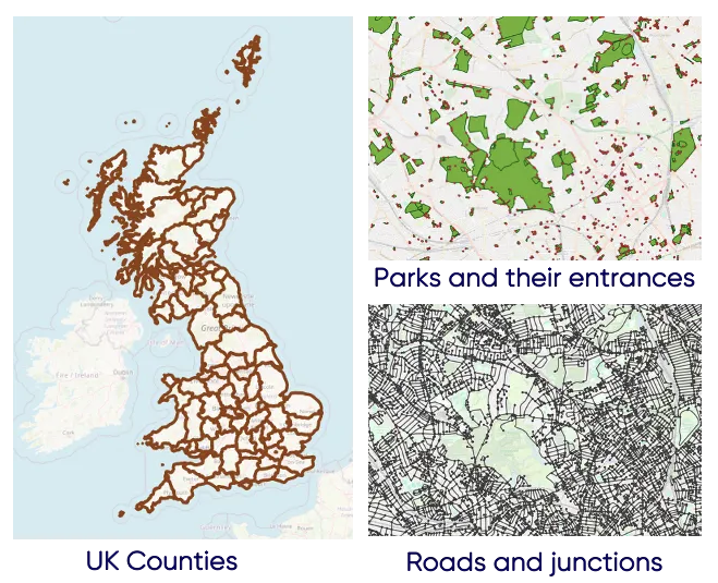
First, I need to gather the relevant datasets. I found the following datasets from the UK Ordnance Survey:
Data design pattern:
Next, from a conceptual perspective, I want to follow the Medallion Architecture (or Multi-hop Architecture). This involves ingesting the raw data as-is (bronze tables), applying filtering, joins, and enrichment (silver tables), and producing the top parks and park entrances (gold table).
Ingestion bronze tables:
Using Apache Sedona, ingestion is quite straightforward. In the code below, you can see how the GeoPackage files are read from an Azure storage account or an AWS S3 bucket:
from sedona.spark import *
from sedona.maps.SedonaPyDeck import SedonaPyDeck
from sedona.maps.SedonaKepler import SedonaKepler
from pyspark.sql import functions as F
from sedona.sql import st_functions as st
from sedona.sql.types import GeometryType
from pyspark.sql.functions import expr


config = SedonaContext.builder() .\
    config('spark.jars.packages',
           'org.apache.sedona:sedona-spark-shaded-3.3_2.12:1.7.1,'
           'org.datasyslab:geotools-wrapper:1.7.1-28.5'). \
    getOrCreate()

sedona = SedonaContext.create(config)


catalog_name = "geospatial"
cloud_provider = "aws"

# Creating a dictionary that specifies the name of the schemas and tables based on the geopackage layers
schema_tables = {
    "lookups": {
        "bdline_gb.gpkg": ["boundary_line_ceremonial_counties"],
    },
    "greenspaces": {
        "opgrsp_gb.gpkg": ["greenspace_site", "access_point"]
    },
    "networks": {
        "oproad_gb.gpkg": ["road_link", "road_node"],
    },
}


# Writing each geopackage layer into a Delta table
for schema, files in schema_tables.items():
    for gpkg_file, layers in files.items():
        for table_name in layers:
            if cloud_provider == "azure":
                df = sedona.read.format("geopackage").option("tableName", table_name).load(f"abfss://{dataset_container_name}@{dataset_storage_account_name}.dfs.core.windows.net/{dataset_dir}/{gpkg_file}")
            elif cloud_provider == "aws":
                df = sedona.read.format("geopackage").option("tableName", table_name).load(f"s3://{dataset_bucket_name}/{dataset_input_dir}/{gpkg_file}")
            df.write.mode("overwrite").saveAsTable(f"{catalog_name}.{schema}.{table_name}")
            print(f"Table {catalog_name}.{schema}.{table_name} is created, yay!")
Explore and visualize:
Now that we have transformed the GeoPackage files into Delta tables with a geometry column, it’s easy and insightful to explore the data and translate business requirements into meaningful code:
%sql
SELECT DISTINCT function
FROM geospatial.greenspaces.greenspace_site
ORDER BY function;
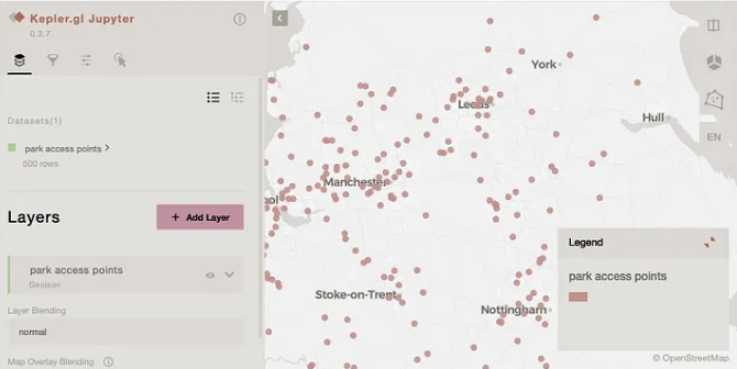
# Reading a Delta table to a spark dataframe
access_point_df  = spark.sql("""
  SELECT fid, access_type, geometry
  FROM geospatial.greenspaces.access_point
  WHERE access_type = 'Pedestrian'
""").limit(500)

# Visualize 500 access points on map using SedonaKepler
map = SedonaKepler.create_map()
SedonaKepler.add_df(map, access_point_df, name="park access points")
map
Enrich silver tables:
With the GeoPackage files now in Delta format, we apply a few enrichments to each table:
1. Using UK administrative boundaries, we distribute the 1000 ice-cream carts based on the area of each region, so that larger areas receive more carts.
# Reading the administrative boundaries and calculating the area
administrative_boundaries  = spark.sql("""
  SELECT b.fid, b.name, ST_Area(b.geometry) AS area, geometry, ST_Geohash(ST_Transform(geometry,'epsg:27700','epsg:4326'), 5) AS geohash
  FROM geospatial.lookups.boundary_line_ceremonial_counties b
""").repartitionByRange(2, "geohash")

total_locations = 1000
uk_arae = administrative_boundaries.selectExpr("SUM(area) AS total_area").first().total_area

# Calculating how many ice-cream carts can be located in each country based on its area
administrative_boundaries = administrative_boundaries.withColumn(
    "number_of_locations",
    F.round(F.col("area") / uk_arae * F.lit(total_locations)).cast("integer")
).orderBy("number_of_locations", ascending=True)

administrative_boundaries.write.mode("overwrite").option("mergeSchema", "true").saveAsTable(f"geospatial.lookups.boundary_line_ceremonial_counties_silver")
administrative_boundaries.createOrReplaceTempView("administrative_boundaries_vw")
2. The greenspace table contains parks, cemeteries, church gardens, etc. We focus on parks. While parks may include playgrounds and other features, we are not interested in the geometries of those smaller areas and the larger park geometry is sufficient. We also categorize parks by size using area quantiles. At the end, we are also interested to know that each parks belong to which county.
# Reading the greenspace_site table and filtering relevant objects
df_greenspaces_bronze = spark.table("geospatial.greenspaces.greenspace_site") \
    .filter("function IN ('Play Space', 'Playing Field', 'Public Park Or Garden')")
df_greenspaces_bronze.createOrReplaceTempView("greenspace_site_bronze_vw")

# Finding the small playgrounds inside larger parks
greenspace_site_covered = spark.sql("""
  SELECT
    g1.id AS g1_id,
    g2.id AS g2_id,
    g1.function AS g1_function,
    g2.function AS g2_function,
    g2.distinctive_name_1 AS g2_name,
    g2.geometry AS geometry,
    ST_Geohash(ST_Transform(g2.geometry ,'epsg:27700','epsg:4326'), 5) AS geohash
  FROM greenspace_site_bronze_vw g1
  INNER JOIN greenspace_site_bronze_vw g2
    ON ST_CoveredBy(g1.geometry, g2.geometry)
   AND g1.id != g2.id
""").repartitionByRange(10, "geohash")

greenspace_site_covered.createOrReplaceTempView("greenspace_site_covered_vw")

# Aggrgating the small playgrounds in the larger parks
greenspace_site_aggregated = spark.sql("""
  SELECT
    g2_id AS id,
    concat_ws(', ', any_value(g2_function), collect_set(g1_function)) AS functions,
    count(*) + 1 AS num_functions,
    g2_name AS name,
    ST_Area(geometry) AS area,
    geometry,
    ST_Geohash(ST_Transform(geometry,'epsg:27700','epsg:4326'), 5) AS geohash
  FROM greenspace_site_covered_vw
  GROUP BY g2_id, g2_name, geometry
""").repartitionByRange(10, "geohash")
greenspace_site_aggregated.createOrReplaceTempView("greenspace_site_aggregated_vw")

# Find the parks without any smaller playgrounds inside them
greenspace_site_non_covered = spark.sql("""
  SELECT id, function, 1 AS num_functions, distinctive_name_1 AS name, ST_Area(geometry) AS area, geometry,
  ST_Geohash(ST_Transform(geometry,'epsg:27700','epsg:4326'), 5) AS geohash
  FROM greenspace_site_bronze_vw
  WHERE id NOT IN (SELECT g1_id FROM greenspace_site_covered_vw)
    AND id NOT IN (SELECT g2_id FROM greenspace_site_covered_vw)
""").repartitionByRange(10, "geohash")
greenspace_site_non_covered.createOrReplaceTempView("greenspace_site_non_covered_vw")

# Union the above two dataframes
greenspace_site_all = spark.sql("""
SELECT * FROM greenspace_site_aggregated_vw
UNION
SELECT * FROM greenspace_site_non_covered_vw""").repartitionByRange(10, "geohash")

# Calculate 0%, 20%, 40%, 60%, 80%, 100% quantiles
quantiles = greenspace_site_all.approxQuantile("area", [0.0, 0.2, 0.4, 0.6, 0.8, 1.0], 0.001)
print("Quintile breakpoints:", quantiles)

q0, q20, q40, q60, q80, q100 = quantiles


# Categorize each park based on its area
greenspace_site_all = greenspace_site_all.withColumn(
    "area_category",
    F.when(F.col("area") <= q20, 20)
     .when(F.col("area") <= q40, 40)
     .when(F.col("area") <= q60, 60)
     .when(F.col("area") <= q80, 80)
     .otherwise(100)
)

display(greenspace_site_all.groupBy("area_category").count().orderBy("area_category"))
greenspace_site_all.createOrReplaceTempView("greenspace_site_all_vw")

# In the final step, we aim to identify the county each park falls within.
greenspace_site_silver = spark.sql("""
WITH tmp AS (
  SELECT a.id, a.functions, a.num_functions, a.name, a.area, a.area_category, a.geometry, a.geohash,
  RANK() OVER(PARTITION BY a.id ORDER BY ST_Area(ST_Intersection(a.geometry, b.geometry)) DESC) AS administrative_rank,
  b.fid as administrative_fid
  FROM greenspace_site_all_vw a
  INNER JOIN administrative_boundaries_vw b
  ON ST_Intersects(a.geometry, b.geometry)
)
SELECT tmp.id, tmp.functions, tmp.num_functions, tmp.name, tmp.area, tmp.area_category, tmp.administrative_fid, tmp.geometry, tmp.geohash
FROM tmp
WHERE  administrative_rank = 1
""").repartitionByRange(10, "geohash")

greenspace_site_silver.createOrReplaceTempView("greenspace_site_silver_vw")

# Write the dataframe into the correspoding silver Delta Table
greenspace_site_silver.write.mode("overwrite").option("mergeSchema", "true").saveAsTable(f"geospatial.greenspaces.greenspace_site_silver")
3. For each road node (i.e. street junction), we calculate the number of edges (streets) connected to it (i.e. the node degree). The more connections, the more prominent the junction.
# Calculate the degree of each road node based on the edges it connects to
road_nodes_silver = spark.sql("""
SELECT a.fid, a.id, a.form_of_road_node, COUNT(DISTINCT b.id) AS degree, a.geometry, ST_Geohash(ST_Transform(a.geometry,'epsg:27700','epsg:4326'), 5) AS geohash
FROM geospatial.networks.road_node a
JOIN geospatial.networks.road_link b
ON a.id = b.start_node
OR a.id = b.end_node
GROUP BY a.fid, a.id, a.form_of_road_node, a.geometry
ORDER BY COUNT(DISTINCT b.id) DESC""").repartitionByRange(10, "geohash")

# Write to a Delta table
road_nodes_silver.write.mode("overwrite").saveAsTable(f"geospatial.networks.road_node_silver")
4. For park entrances, we focus on pedestrian entries, as they attract more foot traffic, ideal for ice-cream carts. We also consider the node degree of the nearest street junction to each entrance, as this reflects how well-connected and accessible the entrance is.
# Find relevant park entrances
greenspace_entries = spark.sql("""
SELECT a.fid, a.id, a.access_type, a.ref_to_greenspace_site, a.geometry, ST_Geohash(ST_Transform(a.geometry,'epsg:27700','epsg:4326'), 5) AS geohash
FROM geospatial.greenspaces.access_point a
WHERE a.ref_to_greenspace_site IN (SELECT id FROM greenspace_site_silver_vw) AND a.access_type IN ('Pedestrian', 'Motor Vehicle And Pedestrian')""").repartitionByRange(10, "geohash")

greenspace_entries.createOrReplaceTempView("greenspace_entries_vw")

# Find its nearest road junction
entry_road_1nn = spark.sql("""
SELECT
    a.fid,
    a.id,
    a.access_type,
    a.ref_to_greenspace_site,
    b.fid AS nearest_road_node_fid,
    ST_Distance(a.geometry, b.geometry) AS distance_to_road_node,
    a.geometry,
    a.geohash
FROM greenspace_entries_vw a
INNER JOIN geospatial.networks.road_node_silver b
ON ST_kNN(a.geometry, b.geometry, 1, FALSE)""").repartitionByRange(10, "geohash")

# Write to a Delta table
entry_road_1nn.write.mode("overwrite").saveAsTable(f"geospatial.greenspaces.access_point_silver")
Aggregated gold tables:
Now that we’ve enriched our silver tables, we can rank each park and entrance based on the defined criteria and select our top 1000 locations.
%sql
-- Top parks to locate the ice-cream carts
CREATE OR REPLACE TABLE geospatial.greenspaces.top_parks_gold AS (
  WITH tmp AS (
    SELECT
    gs.id,
    gs.name AS park_name,
    gs.functions,
    gs.num_functions,
    gs.area_category,
    sum(rn.degree) AS accessibility_degree,
    cc.name AS county,
    cc.number_of_locations,
    row_number() OVER (PARTITION BY cc.name ORDER BY gs.area_category DESC, gs.num_functions DESC, sum(degree) DESC) AS park_rank,
    ST_AsEWKB(gs.geometry) AS geometry
    FROM geospatial.greenspaces.greenspace_site_silver gs
    LEFT JOIN geospatial.greenspaces.access_point_silver ga
    ON gs.id = ga.ref_to_greenspace_site
    LEFT JOIN geospatial.networks.road_node_silver rn
    ON ga.nearest_road_node_fid = rn.fid
    LEFT JOIN geospatial.lookups.boundary_line_ceremonial_counties_silver cc
    ON gs.administrative_fid = cc.fid
    GROUP BY gs.name, gs.functions, gs.num_functions, gs.area_category, cc.number_of_locations, cc.name, gs.geometry, gs.id, cc.name)
  SELECT * FROM tmp WHERE park_rank <= number_of_locations);
%sql
-- Top entrances to locate the ice-cream carts
CREATE OR REPLACE TABLE geospatial.greenspaces.top_entrances_gold AS (
  WITH A AS (
    SELECT
    ga.id,
    ga.ref_to_greenspace_site AS park_id,
    gs.park_rank,
    ga.access_type,
    rn.degree,
    ga.distance_to_road_node,
    row_number() OVER (PARTITION BY gs.id ORDER BY rn.degree DESC, ga.distance_to_road_node ASC) AS entry_rank,
    ST_AsEWKB(ga.geometry) AS geometry,
    ST_X(ST_Transform(ga.geometry,'epsg:27700','epsg:4326')) AS longitude,
    ST_Y(ST_Transform(ga.geometry,'epsg:27700','epsg:4326')) AS latitude
    FROM geospatial.greenspaces.top_parks_gold gs
    LEFT JOIN geospatial.greenspaces.access_point_silver ga
    ON gs.id = ga.ref_to_greenspace_site
    LEFT JOIN geospatial.networks.road_node_silver rn
    ON ga.nearest_road_node_fid = rn.fid
  )
  SELECT * FROM A WHERE entry_rank = 1
);
What is next?
In our live training “Databricks Geospatial in a Day” at RevoData Office, we’ll delve deeper into the logic behind this code and use this example to demonstrate how to:
· Set up a cluster with all necessary geospatial libraries
· Follow best practices for working with Unity Catalog
· Organize data using the Medallion Architecture
· Build an orchestration workflow
· Create an AI/BI dashboard to visualize the top entrances

Melika Sajadian
Senior Geospatial Consultant at RevoData, sharing with you her knowledge about Databricks Geospatial