Editor’s note: This post was originally published June 12th, 2025.
What is environmental change detection?
Think of it as a time machine for planet Earth. No flux capacitor, no DeLorean, and no Marty McFly needed!😉 Just some cool tech that lets us peek into how our world changes over time.
Detecting and understanding environmental changes is essential for informed decision-making, sustainable development, and effective disaster risk reduction. By systematically identifying and monitoring trends such as deforestation, urban expansion, and coastal erosion at an early stage, policymakers, urban planners, environmental agencies, and other relevant stakeholders can implement timely and proactive measures to mitigate adverse impacts on ecosystems, biodiversity, and vulnerable human populations.
Change detection provides a critical evidence base for assessing the effectiveness of existing environmental policies and conservation strategies. It also plays a key role in informing the planning and development of resilient infrastructure capable of withstanding future environmental stresses. Furthermore, by offering accurate and up-to-date information, it supports more efficient resource allocation and helps prioritize areas facing the greatest risks.
Above all, the ability to detect and interpret environmental changes enhances society’s capacity to respond to climate-related challenges such as sea-level rise, extreme weather events, and habitat degradation. In this context, change detection serves as a vital tool for promoting more responsible and adaptive management of the planet in an era marked by rapid and often unpredictable transformation. While this “time machine” can’t rewrite history, it empowers us to learn from the past and chart a course toward a more sustainable future.
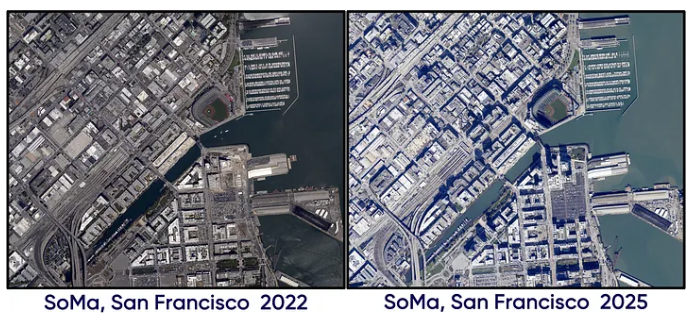
For today’s adventure, I’m using Databricks and Apache Sedona , they’re basically the power tools for working with geospatial data without your computer having a meltdown. And where are we headed? San Francisco,specifically the SoMa (South of Market) area! We’re gonna see how it looked in August 2022 versus February 2025. Trust me, even in just a couple years, you’d be surprised how much a neighborhood can transform. It’s like watching your city grow up in fast-forward.
Implementation
The following implementation is part of the training we offer at RevoData focused specifically on leveraging the geospatial capabilities of Databricks.
Remote sensing and photogrammetry cover a lot of ground, you’ve got active and passive sensors, different types of resolution (spatial, spectral, temporal, radiometric), geo-referencing, orthophoto generation, and electromagnetic spectrum analysis. Instead of getting bogged down in all the technical details, I’m going to focus on why I chose certain methods and what other options could potentially be considered. Let’s get started.
Datasets
First things first, we need data, but what kind? For change detection in an urban environment, we typically rely on satellite or aerial images captured in at least four spectral bands: Red, Green, Blue, and Near Infrared (NIR). Why NIR? Well, it all comes down to physics. Different sensors detect different ‘flavors’ of energy, from visible light our eyes see to invisible infrared or microwave radiation. Each sensor type reveals unique information about Earth’s surface based on the specific energy waves it can measure. What the sensor ‘sees’ depends on how objects interact with these waves:
- Absorption: The surface soaks up the energy (like dark pavement heating in sunlight)
- Reflection: The energy bounces back (like light mirroring off a lake)
- Transmission: The energy passes through (like sunlight through clear water)
Different materials, such as water, soil, concrete, vegetation, each have unique ‘fingerprints’ in how they handle these waves. That’s how we can identify and monitor features from satellites or aircraft!
These interactions allow us to calculate indices such as the Normalized Difference Vegetation Index (NDVI) and the Normalized Difference Water Index (NDWI). These are simple and useful for classifying each image pixel as vegetation, water, or bare ground. You can also go a step further and apply machine learning or pattern recognition algorithms, like the maximum likelihood classifier, to identify different phenomena across the landscape.
The good news? This kind of imagery is freely available. You can easily access the data in GeoTiff format through the NOAA Data Access Viewer and begin your own journey through space and time.
Data ingestion
Once again, Apache Sedona makes geospatial data ingestion remarkably easy.
					from pyspark.sql.functions import expr, explode, col
from sedona.spark import *
from pyspark.sql.window import Window
from pyspark.sql import functions as F
from pyspark.sql import SparkSession

config = SedonaContext.builder() .\
    config('spark.jars.packages',
           'org.apache.sedona:sedona-spark-shaded-3.3_2.12:1.7.1,'
           'org.datasyslab:geotools-wrapper:1.7.1-28.5'). \
    getOrCreate()

sedona = SedonaContext.create(config)


file_urls = {"2022": f"s3://{dataset_bucket_name}/geospatial-dataset/raster/orthophoto/soma/2022/2022_4BandImagery_SanFranciscoCA_J1191044.tif",
              "2025": f"s3://{dataset_bucket_name}/geospatial-dataset/raster/orthophoto/soma/2025/2025_4BandImagery_SanFranciscoCA_J1191043.tif"}

df_image_2025 = sedona.read.format("binaryFile").load(file_urls["2025"])
df_image_2025 = df_image_2025.withColumn("raster", expr("RS_FromGeoTiff(content)"))

df_image_2022 = sedona.read.format("binaryFile").load(file_urls["2022"])
df_image_2022 = df_image_2022.withColumn("raster", expr("RS_FromGeoTiff(content)"))
Exploring the data
We can retrieve metadata from the 2025 image by executing the following query:
df_image_2025.createOrReplaceTempView("image_new_vw")
display(spark.sql("""SELECT RS_MetaData(raster) AS metadata,
                  RS_NumBands(raster) AS num_bands,
                  RS_SummaryStatsAll(raster) AS summary_stat,
                  RS_BandPixelType(raster) AS band_pixel_type,
                  RS_Count(raster) AS count
                  FROM image_new_vw"""))
Tiling for scalable image analysis
To improve scalability and enhance performance in the upcoming analysis, we first tile the image into smaller segments:
tile_w = 195
tile_h = 191

tiled_df_2025 = df_image_2025.selectExpr(
  f"RS_TileExplode(raster, {tile_w}, {tile_h})"
).withColumnRenamed("x", "tile_x").withColumnRenamed("y", "tile_y").withColumn("width", expr("RS_Width(tile)")).withColumn("height", expr("RS_height(tile)"))
window_spec = Window.orderBy("tile_x", "tile_y")
tiled_df_2025 = tiled_df_2025.withColumn("rn", F.row_number().over(window_spec)).withColumn("year", lit(2025))

tiled_df_2022 = df_image_2022.selectExpr(
  f"RS_TileExplode(raster, {tile_w}, {tile_h})"
).withColumnRenamed("x", "tile_x").withColumnRenamed("y", "tile_y").withColumn("width", expr("RS_Width(tile)")).withColumn("height", expr("RS_height(tile)"))
window_spec = Window.orderBy("tile_x", "tile_y")
tiled_df_2022 = tiled_df_2022.withColumn("rn", F.row_number().over(window_spec)).withColumn("year", lit(2022))

union_raster = tiled_df_2022.unionByName(tiled_df_2025, allowMissingColumns=False)
window_spec = Window.partitionBy("rn").orderBy(F.desc("year"))
union_raster = union_raster.withColumn("index", F.row_number().over(window_spec))
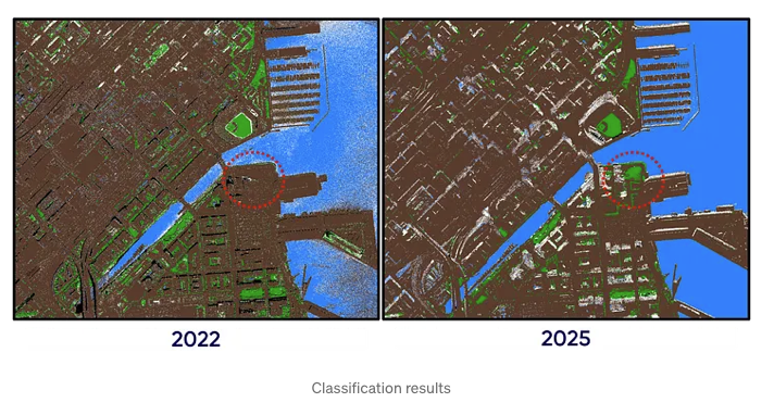
Image classification
We perform pixel-wise classification by calculating the NDVI and NDWI indices and applying a simple decision tree. The classification criteria are informed not only by the definitions of NDVI and NDWI, but also by temporal differences between the two images, which were captured at different times of the year and day. These differences are observable, for instance, in the varying shadows cast by buildings. As with any classification approach, some degree of misclassification is expected. Then the results are written to a Delta table.
					# Calculating NDVI using Red and NIR bands as NDVI = (NIR - Red) / (NIR + Red)
union_raster = union_raster.withColumn(
    "ndvi",
    expr(
        "RS_Divide("
        "  RS_Subtract(RS_BandAsArray(tile, 1), RS_BandAsArray(tile, 4)), "
        "  RS_Add(RS_BandAsArray(tile, 1), RS_BandAsArray(tile, 4))"
        ")"
    )
)


# Calculating NDWI using Green and NIR bands as NDWI = (Green - NIR) / (Green + NIR)
union_raster = union_raster.withColumn(
    "ndwi",
    expr(
        "RS_Divide("
        "  RS_Subtract(RS_BandAsArray(tile, 4), RS_BandAsArray(tile, 2)), "
        "  RS_Add(RS_BandAsArray(tile, 4), RS_BandAsArray(tile, 2))"
        ")"
    )
)

# Red and Green bands as arrays in new columns
union_raster = union_raster.withColumn(
    "red",
    expr(
        "RS_BandAsArray(tile, 1)"
    )
).withColumn(
    "green",
    expr(
        "RS_BandAsArray(tile, 2)"
    )
)


# Classification tree based on Red and Green bands and NDVI, NDWI
union_raster = union_raster.withColumn(
    "classification",
    F.expr("""
        transform(
            arrays_zip(ndvi, ndwi, red, green),
            x ->
                CASE
                    WHEN year = 2022 THEN
                        CASE
                            WHEN x.red < 15 AND x.green < 15 THEN 4
                            WHEN x.ndvi > 0.35 AND x.ndwi < -0.35 THEN 2
                            WHEN (x.ndvi < -0.2 AND x.ndwi > 0.35) OR (x.red < 15 AND x.ndwi > 0.35) OR (x.ndwi > 0.45) THEN 3
                            WHEN x.ndvi >= -0.3 AND x.ndvi <= 0.3 AND x.ndwi >= -0.3 AND x.ndwi <= 0.3 THEN 1
                            ELSE 999
                        END
                    WHEN year = 2025 THEN
                        CASE
                            WHEN x.red < 15 AND x.green < 15 THEN 4
                            WHEN x.ndvi > 0.3 AND x.ndwi < -0.15 THEN 2
                            WHEN x.ndvi < -0.35 AND x.ndwi > 0.55 THEN 3
                            WHEN (x.ndvi >= -0.5 AND x.ndvi <= 0.5 AND x.ndwi >= -0.5 AND x.ndwi <= 0.5) OR (x.ndvi > 0.8 AND x.ndwi > 0.3) THEN 1
                            ELSE 999
                        END
                    ELSE 999
                END
        )
    """)
)

# Classification array as a new band in the raster and defining no data value as 999
classification_df = (
    union_raster
    .select("tile_x", "tile_y", "rn", "year", "index", expr("RS_MakeRaster(tile, 'I', classification) AS tile").alias("tile"))
    .select("tile_x", "tile_y", "rn", "year", "index", expr("RS_SetBandNoDataValue(tile,1, 999, false)").alias("tile"))
    .select("tile_x", "tile_y", "rn", "year", "index", expr("RS_SetBandNoDataValue(tile,1, 999, true)").alias("tile"))
)

classification_df = classification_df.withColumn("maxValue", expr("""RS_SummaryStats(tile, "max", 1, false)"""))

classification_df.withColumn("raster_binary", expr("RS_AsGeoTiff(tile)")).select("tile_x", "tile_y","rn", "year", "index", "raster_binary").write.mode("overwrite").saveAsTable("geospatial.soma.classification")
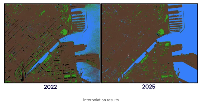
Filling missing data via interpolation
In the images above, we can observe white areas, i.e. pixels that couldn’t be classified and were left as no-data values. To address this, we can apply interpolation using the Inverse Distance Weighting (IDW) method. Apache Sedona simplifies this process: we filter out the tiles with no-data values and perform the interpolation. After that, we store the interpolated results in a Delta table.
# Separating the dataframe into two dataframes based on the
no_interpolation_df = classification_df.filter(classification_df["maxValue"] != 999).select("tile_x", "tile_y","rn", "year", "index", "raster_binary")
interpolated_df = classification_df.filter(classification_df["maxValue"] == 999).select("tile_x", "tile_y","rn", "year", "index", expr("RS_Interpolate(tile, 2.0, 'variable', 48.0, 6.0)").alias("tile")).withColumn("raster_binary", expr("RS_AsGeoTiff(tile)")).select("tile_x", "tile_y","rn", "year", "index", "raster_binary")
union_df = interpolated_df.unionByName(no_interpolation_df, allowMissingColumns=False)
union_df.write.mode("overwrite").saveAsTable("geospatial.soma.interpolation")
union_df = spark.table("geospatial.soma.interpolation").withColumn("tile", expr("RS_FromGeoTiff(raster_binary)"))
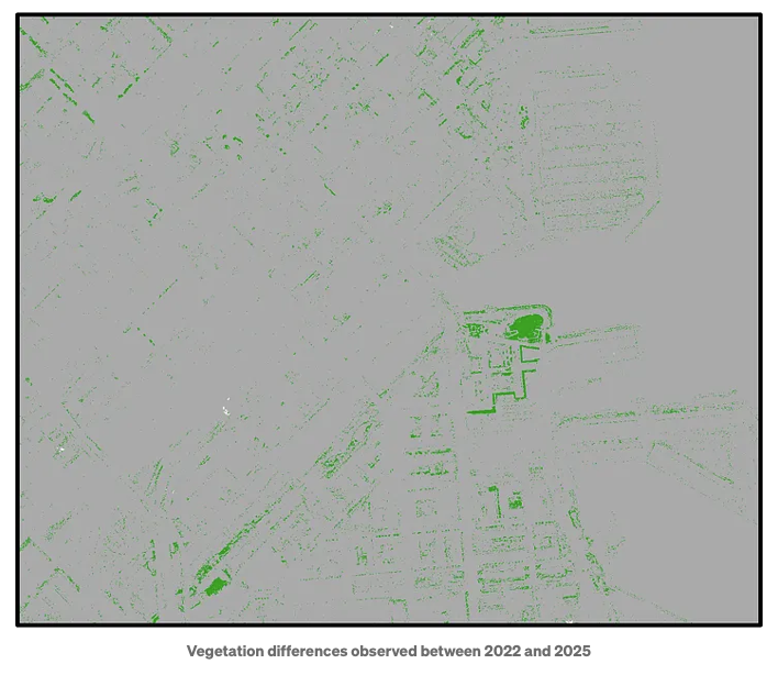
Evaluating classification changes between the two images
It would be useful to create a band that highlights the differences between the classifications from 2022 and 2025, and add it as the third band in the image.
union_df.createOrReplaceTempView("union_df_vw")

merged_raster = sedona.sql("""
    SELECT rn, RS_Union_Aggr(tile, index) AS raster
    FROM union_df_vw
    GROUP BY rn
""")

merged_raster.createOrReplaceTempView("merged_raster_vw")
diff_raster = merged_raster.withColumn("diff_band", expr(
        "RS_LogicalDifference("
        "RS_BandAsArray(raster, 1), RS_BandAsArray(raster, 2)"
        ")"))

result_df = diff_raster.select("rn", expr("RS_AddBandFromArray(raster, diff_band) AS raster").alias("raster")).withColumn("raster_binary", expr("RS_AsGeoTiff(raster)"))
result_df.select("rn", "raster_binary").write.mode("overwrite").saveAsTable("geospatial.soma.change_detection")
Finally, we can detect and visualize changes, such as those in vegetation, using the image below as an example:
What is next?
In our live training “Databricks Geospatial in a Day” at RevoData Office, we’ll delve deeper into the logic behind this code and use this example to demonstrate how to:
- Visualize GeoTIFF files
- Generate optimally sized tiles from large raster datasets
- Configure clusters optimized for compute-intensive workloads, such as spatial interpolation
- Partition Spark DataFrames by the raster column to accelerate processing
- Use complementary tools to seamlessly merge tiles back into a single large GeoTIFF
Go ahead and grab your spot for the training using the link below, can’t wait to see you there!
https://revodata.nl/databricks-geospatial-in-a-day/

Melika Sajadian
Senior Geospatial Consultant at RevoData, sharing with you her knowledge about Databricks Geospatial