Editor’s note: This post was originally published June 20th, 2025.
What is the Sky View Factor and why does it matter in our cities?
I’m back with another sunny, summer-inspired geospatial adventure!
Ever wonder how much sky you can actually see when you’re standing on a busy city street or under a cluster of city trees? That visible slice of sky called the Sky View Factor (SVF) has a surprisingly big say in how cities heat up, cool down, and even how comfortable we feel outside. The less sky you see, the more heat gets trapped between buildings and trees, creating those urban heat islands, where city temperatures climb higher than surrounding areas. These heat islands don’t just make summer days unbearable, they can worsen air pollution, increase energy demand for cooling, strain public health by amplifying heat-related illnesses, and even accelerate the wear and tear on city infrastructure.
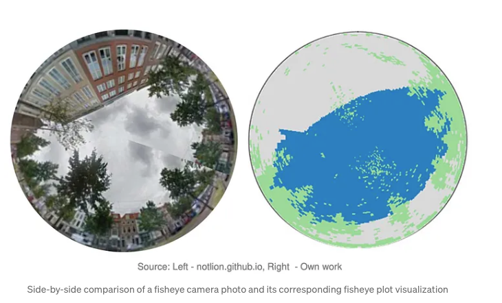
Measuring SVF takes more than just a weather app or a quick satellite snapshot, you need a detailed, 3D, street-level view of the city. That’s where LiDAR point cloud data shines, capturing billions of laser-scanned points from every rooftop, treetop, street, and sidewalk. This treasure trove of 3D data lets us model the urban canopy, the intricate layer of buildings and greenery that controls how sunlight and air flow through the cityscape. From this, we can calculate SVF and generate cool fisheye plots that show exactly how much sky you’d see lying anywhere on the ground.
Back in my master’s program, some classmates and I built an app for the municipality of The Hague that let users click on a map or upload a list of points to get SVF values and how much the sky is blocked by buildings and trees. You can check out our full report with the front-end and backend code here. Back then, we ran the calculations using NumPy arrays and plenty of good old-fashioned for-loops. I’m now reworking the project using PySpark, with a focus on scalable, data warehousing for big data analytics rather than real-time, on-the-fly processing, without delving deeply into the underlying mathematical computations. That’s where Databricks shines: its cloud-native platform effortlessly handles massive LiDAR datasets, turning mountains of 3D points into quick, actionable insights. Whether you’re a city planner aiming to cool down urban streets or simply a curious urban data explorer, it’s never been easier or more fun to look up and ask: how much sky do we really see?
Implementation:
The following implementation is part of the training we offer at RevoData focused specifically on leveraging the geospatial capabilities of Databricks.
In this implementation, I want to focus on code refactoring and explore the options available to start with the low-hanging fruit, highlighting which parts of the code can be adapted for distributed processing with minimal changes.
Let’s get started!
Datasets
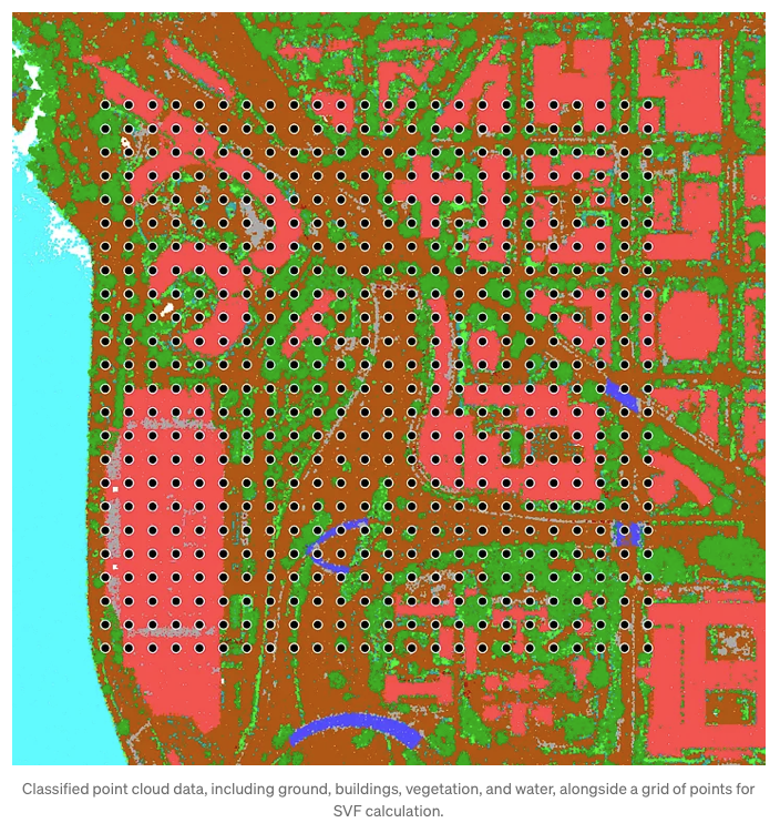
As I mentioned earlier, we originally used point cloud data from the City of The Hague for this project. But today, I’m taking you to Washington, partly to switch up the scenery for myself, and partly so you can download the data more easily from an English-language website. The data is fully available here. I also generated a grid of 576 points across the area, which we’ll use to calculate the Sky View Factor (SVF).
Import libraries
In this implementation, we need couple of libraries which I import in one go:
					import math
import numpy as np
import boto3
import os
import matplotlib.pyplot as plt
import pdal
import json
import io
import pyarrow as pa
from pyspark.sql.functions import col, sqrt, pow, lit, when, atan2, degrees, floor
from pyspark.sql.types import StructType, StructField, DoubleType, FloatType, IntegerType, ShortType, LongType, ByteType, BooleanType, MapType, StringType, ArrayType
import pandas as pd
from sedona.spark import *
from pyspark.sql import functions as F
from pyspark.sql.window import Window
import base64
from PIL import Image
Data ingestion
For the generated grid points, Apache Sedona makes geospatial data ingestion remarkably easy.
config = SedonaContext.builder() .\
    config('spark.jars.packages',
           'org.apache.sedona:sedona-spark-shaded-3.3_2.12:1.7.1,'
           'org.datasyslab:geotools-wrapper:1.7.1-28.5'). \
    getOrCreate()

sedona = SedonaContext.create(config)

# The path to the grid geopackage and point cloud las file
dataset_bucket_name = "revodata-databricks-geospatial"
dataset_input_dir="geospatial-dataset/point-cloud/washington"
gpkg_file = "grid/pc_grid.gpkg"
pointcloud_file = "las-laz/1816.las"
input_path = f"s3://{dataset_bucket_name}/{dataset_input_dir}/{pointcloud_file}"

# Read the grid data
df_grid = sedona.read.format("geopackage").option("tableName", "grid").load(f"s3://{dataset_bucket_name}/{dataset_input_dir}/{gpkg_file}").withColumnRenamed("geom", "geometry").withColumn("x1", F.expr("ST_X(geometry)")).withColumn("y1", F.expr("ST_Y(geometry)")).select("fid", "x1", "y1", "geometry")

num_partitions = math.ceil(df_grid.count()/2)
To ingest point cloud data, we can use libraries like laspy or PDAL. In this case, I used PDAL, applying a few read-time optimizations to efficiently convert the output array into a PySpark DataFrame:
def _create_arrow_schema_from_pdal(pdal_array):
    """Create Arrow schema from PDAL array structure."""
    fields = []

    # Map PDAL types to Arrow types
    type_mapping = {
        'float32': pa.float32(),
        'float64': pa.float64(),
        'int32': pa.int32(),
        'int16': pa.int16(),
        'uint8': pa.uint8(),
        'uint16': pa.uint16(),
        'uint32': pa.uint32()
    }

    for field_name in pdal_array.dtype.names:
        field_type = pdal_array[field_name].dtype
        arrow_type = type_mapping.get(str(field_type), pa.float32())  # default to float32
        fields.append((field_name, arrow_type))

    return pa.schema(fields)

def _create_spark_schema(arrow_schema):
    """Convert PyArrow schema to Spark DataFrame schema."""
    spark_fields = []

    type_mapping = {
        pa.float32(): FloatType(),
        pa.float64(): DoubleType(),
        pa.int32(): IntegerType(),
        pa.int16(): ShortType(),
        pa.int8(): ByteType(),
        pa.uint8(): ByteType(),
        pa.uint16(): IntegerType(),  # Spark doesn't have unsigned types
        pa.uint32(): LongType(),     # Spark doesn't have unsigned types
        pa.string(): StringType(),
        # Add other type mappings as needed
    }

    for field in arrow_schema:
        arrow_type = field.type
        spark_type = type_mapping.get(arrow_type, StringType())  # default to StringType
        spark_fields.append(
            StructField(field.name, spark_type, nullable=True)
        )

    return StructType(spark_fields)


def pdal_to_spark_dataframe_large(pipeline_config, spark, chunk_size=1000000):
    """Streaming version for very large files."""
    pipeline = pdal.Pipeline(json.dumps(pipeline_config))
    pipeline.execute()

    # Get schema from first array
    first_array = pipeline.arrays[0]
    schema = _create_arrow_schema_from_pdal(first_array)

    # Create empty RDD
    rdd = spark.sparkContext.emptyRDD()


    # Process arrays in chunks
    for array in pipeline.arrays:
        for i in range(0, len(array), chunk_size):
            chunk = array[i:i+chunk_size]
            data_dict = {name: chunk[name] for name in chunk.dtype.names}
            arrow_table = pa.Table.from_pydict(data_dict, schema=schema)
            pdf = arrow_table.to_pandas()
            chunk_rdd = spark.sparkContext.parallelize(pdf.to_dict('records'))
            rdd = rdd.union(chunk_rdd)

    # Convert to DataFrame
    return spark.createDataFrame(rdd, schema=_create_spark_schema(schema))
pipeline_config = {
    "pipeline": [
        {
            "type": "readers.las",
            "filename": input_path,
        }
    ]
}

# Convert point cloud array to Spark DataFrame
df_pc = pdal_to_spark_dataframe_large(pipeline_config, spark)
df_pc = df_pc.withColumn("geometry", F.expr("ST_Point(X, Y)"))
df_pc.write.mode("overwrite").saveAsTable(f"geospatial.pointcloud.wasahington_pc")
Identifying point cloud data surrounding each grid point
Next, we need to retrieve all point cloud data within 100 meters for buildings and high vegetation, these are used for SVF calculation. For ground points, we only consider those within 10 meters, as they’re used solely to estimate the elevation of each grid point.
					df_selected = df_pc.select("X", "Y", "Z", "Classification")

dome_radius = 100
height_radius = 10

# Register as temp views
df_pc.createOrReplaceTempView("pc_vw")
df_grid.createOrReplaceTempView("grid_vw")

# Perform spatial join using ST_DWithin with 100 meters
grid_join_pc = spark.sql(f"""
    SELECT
        g.fid,
        ST_X(g.geometry) AS x1,
        ST_Y(g.geometry) AS y1,
        p.classification,
        p.x AS pc_x,
        p.y AS pc_y,
        p.z AS pc_z,
        ST_Distance(g.geometry, p.geometry) AS distance,
        g.geometry AS g_geometry,
        p.geometry AS pc_geometry
    FROM grid_vw g
    JOIN pc_vw p
        ON ST_DWithin(g.geometry, p.geometry, {dome_radius})
    WHERE p.classification IN (5, 6) OR (p.classification = 2 AND ST_DWithin(g.geometry, p.geometry, {height_radius}))
""")
Estimating grid point elevation from nearby point cloud data (10m Radius)
Here, we determine the elevation of each grid point by identifying its dominant surrounding class, either building or ground, and then computing the average elevation of that class within a defined radius.
					# Filter only classification 2 and 6 and count occurrences of (fid, classification)
grouped = grid_join_pc.filter(
    (F.col("classification").isin(2, 6)) & (F.col("distance") <= height_radius)
).groupBy("fid", "classification").count()

# Define window: partition by fid, order by count descending
window_spec = Window.partitionBy("fid").orderBy(F.desc("count"))

# Apply row_number
ranked = grouped.withColumn("rn", F.row_number().over(window_spec))

# Compute the average elevation for each grid point using nearby point cloud data within a specified radius.
grid_pc_elevation = grid_join_pc.join(g_classification_df, on=["fid", "classification"]).filter(
    (F.col("distance") <= height_radius)
).groupBy("fid").agg(
    (F.sum("pc_z") / F.count("pc_z")).alias("height")
)

# Combine point cloud data with classification info and computed height, optimized with repartitioning.
grid_pc_elevation_all = grid_join_pc.withColumnRenamed("classification", "p_classification").join(g_classification_df, on=["fid"]).join(grid_pc_elevation, on=["fid"]).repartitionByRange(num_partitions, "fid")

# Filter out ground points (e.g., class 2) to retain only buildings and high vegetation points for analysis.
grid_pc_cleaned = grid_pc_elevation_all.filter("p_classification != 2").repartitionByRange(num_partitions, "fid")
Creating the dome, generating the plot, and calculating the SVF
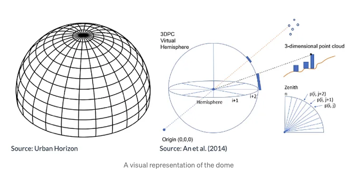
The dome is a representation of the sky, going from the horizon all the way to the zenith (directly on top) of the viewpoint. The dome can be split into sectors based on horizontal and vertical directions, in essence creating a dome-like shaped grid. The units used to split the sectors are 2 degrees horizontally (azimuth angle), and 1 degree vertically (elevation angle), which are considered as appropriate values for calculation.
To calculate the Sky View Factor (SVF), point cloud data is projected onto a dome divided into sectors, marking which sectors are blocked from view. The closest point in each sector determines the obstruction, and if that point is a building, all sectors below it in that direction are also considered blocked. The unobstructed proportion of the dome’s area gives the SVF. For clarity, the results are visualized in a circular plot showing which sectors are clear sky or obstructed by buildings or vegetation, oriented to the north for easy interpretation.
					# Calculate raw azimuth angle (in degrees) from each grid point to each point in the point cloud.
# Shifted by -90 to align with the 0° direction being north.
grid_pc_az = grid_pc_cleaned.withColumn(
    "azimuth_raw",
    degrees(F.atan2(F.col("pc_y") - F.col("y1"), F.col("pc_x") - F.col("x1"))) - 90
)

# Normalize azimuth angle to fall within the range [0, 360).
grid_pc_az = grid_pc_az.withColumn(
    "azimuth",
    when(F.col("azimuth_raw") < 0, F.col("azimuth_raw") + 360).otherwise(F.col("azimuth_raw"))
)

# Drop the temporary azimuth_raw column to clean up the DataFrame.
grid_pc_az = grid_pc_az.drop("azimuth_raw")

# Calculate the elevation angle (in degrees) from the grid point to each point in the point cloud.
# Height is divided by 1000 to convert from millimeters to meters if necessary.
grid_pc_az = grid_pc_az.withColumn(
    "elevation",
    degrees(F.atan2(F.col("pc_z") - F.col("height") / 1000, F.col("distance")))
)

# Bin azimuth angles into 2-degree intervals (0–179 bins for 360°).
grid_pc_az = grid_pc_az.withColumn("azimuth_bin", F.floor(F.col("azimuth") / 2))

# Get the minimum elevation angle across all records to define the lower bound of elevation bins.
min_val = F.lit(grid_pc_az.select(F.min("elevation")).first()[0])

# Get the maximum elevation angle across all records to define the upper bound of elevation bins.
max_val = F.lit(grid_pc_az.select(F.max("elevation")).first()[0])

# Compute bin width by dividing elevation range into 89 equal parts (90 bins total).
bin_width = (max_val - min_val) / 89

# Bin elevation angles into 90 intervals, ensuring they stay within the [0, 89] range.
grid_pc_az = grid_pc_az.withColumn("elevation_bin",
    F.least(
        F.greatest(
            F.floor(
                (F.col("elevation") - F.lit(min_val)) /
                F.lit((max_val - min_val)/90)
            ).cast("int"),
            F.lit(0)  # Clamp minimum bin index to 0
        ),
        F.lit(89)  # Clamp maximum bin index to 89
    )
)


# Define a window that partitions the data by azimuth and elevation bins,
# and orders points within each bin by their distance to the grid point.
window_spec = Window.partitionBy("azimuth_bin", "elevation_bin").orderBy("distance")

# Assign a row number within each azimuth-elevation bin, so the closest point (smallest distance) gets rank 1.
df_with_rank = grid_pc_az.withColumn("rn", F.row_number().over(window_spec))

# Keep only the closest point (rank 1) in each bin and drop the temporary rank column.
# Then repartition the result by 'fid' to optimize parallel processing in subsequent steps.
closest_points = df_with_rank.filter(col("rn") == 1).drop("rn").repartitionByRange(num_partitions, "fid")
def create_dome(pdf: pd.DataFrame, max_azimuth: int = 180, max_elevation: int = 90) -> np.ndarray:
    """
    Creates a dome matrix based on azimuth and elevation bins, with obstruction handling for buildings.
    """
    dome = np.zeros((max_azimuth, max_elevation), dtype=int)
    domeDists = np.zeros((max_azimuth, max_elevation), dtype=float)

    for _, row in pdf.iterrows():
        a = int(row["azimuth_bin"])
        e = int(row["elevation_bin"])
        dome[a, e] = row["p_classification"]
        domeDists[a, e] = row["distance"]

    # Mark parts of the dome that are obstructed by buildings
    if np.any(dome == 6):  # 6 = buildings
        bhor, bver = np.where(dome == 6)
        builds = np.stack((bhor, bver), axis=-1)
        shape = (builds.shape[0] + 1, builds.shape[1])
        builds = np.append(builds, (bhor[0], bver[0])).reshape(shape)
        azimuth_change = builds[:, 0][:-1] != builds[:, 0][1:]
        keep = np.where(azimuth_change)
        roof_rows, roof_cols = builds[keep][:, 0], builds[keep][:, 1]
        for roof_row, roof_col in zip(roof_rows, roof_cols):
            condition = np.where(np.logical_or(
                domeDists[roof_row, :roof_col] > domeDists[roof_row, roof_col],
                dome[roof_row, :roof_col] == 0
            ))
            dome[roof_row, :roof_col][condition] = 6

    return dome

# Plot dome
def generate_plot_image(dome):
    # Create circular grid
    theta = np.linspace(0, 2*np.pi, 180, endpoint=False)
    radius = np.linspace(0, 90, 90)
    theta_grid, radius_grid = np.meshgrid(theta, radius)

    Z = dome.copy().astype(float)

    Z = Z.T[::-1, :]  # Transpose and flip vertically

    Z[Z == 0] = 0
    Z[np.isin(Z, [5])] = 0.5
    Z[Z == 6] = 1

    if Z[Z == 6].size == 0:
        Z[0, 0] = 1  # Force plot to show something

    fig = plt.figure(figsize=(4, 4))
    ax = fig.add_subplot(111, projection='polar')
    cmap = plt.get_cmap('tab20c')
    ax.pcolormesh(theta, radius, Z, cmap=cmap)
    ax.set_ylim([0, 90])
    ax.tick_params(labelleft=False)
    ax.set_theta_zero_location("N")
    ax.set_xticks([])
    ax.set_yticks([])

    buf = io.BytesIO()
    plt.savefig(buf, format='png', bbox_inches='tight', pad_inches=0)
    plt.close(fig)
    buf.seek(0)
    img_base64 = base64.b64encode(buf.read()).decode('utf-8')
    return img_base64


def process_and_plot(pdf: pd.DataFrame) -> pd.DataFrame:
    fid = pdf["fid"].iloc[0]

    # Create dome with building/vegetation obstruction
    dome = create_dome(pdf)

    # Generate base64-encoded fisheye plot image
    plot_base64 = generate_plot_image(dome)

    # Compute SVF and obstruction metrics
    SVF, tree_percentage, build_percentage = calculate_SVF(100, dome)

    return pd.DataFrame(
        [[fid, dome.tolist(), plot_base64, SVF, tree_percentage, build_percentage]],
        columns=["fid", "dome", "plot", "SVF", "treeObstruction", "buildObstruction"]
    )
Results
As you can see in the code above, some parts still rely on NumPy structures for operations like dome construction, plotting and SVF calculation. Since each grid point corresponds to a single dome, we can safely apply these NumPy-based functions on a per-row basis. To do this efficiently in PySpark , without too much code refactoring, I use the applyInPandas method. This allows us to apply our existing Pandas-based logic directly to each group of rows (grouped by the "fid" column) within the PySpark DataFrame. This way, we can leverage distributed processing in Spark while reusing existing, well-tested NumPy code for the dome and SVF calculations.
					# Desired schema
output_schema = StructType([
    StructField("fid", IntegerType()),
    StructField("dome", ArrayType(ArrayType(IntegerType()))),
    StructField("plot", StringType()),
    StructField("SVF", FloatType()),
    StructField("treeObstruction", FloatType()),
    StructField("buildObstruction", FloatType())
])

result_df = closest_points.groupBy("fid").applyInPandas(process_and_plot, schema=output_schema)
result_df.write.mode("overwrite").saveAsTable(f"geospatial.pointcloud.wasahington_grid")
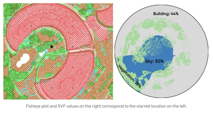
# Fetch the the grid point with fid = 105 for a sample visualization
pdf = result_df.filter("fid = 105").select("fid", "plot").toPandas()

for index, row in pdf.iterrows():
  # Decode base64 string to bytes
  img_bytes = base64.b64decode(img_base64)

  # Load image with PIL
  image = Image.open(io.BytesIO(img_bytes))

  # Display using matplotlib (preserves original colors)
  plt.figure(figsize=(6, 6))
  plt.imshow(image)
  plt.axis('off')  # Hide axes
  plt.show()
What is next?
In our live training “Databricks Geospatial in a Day” at RevoData Office, we’ll delve deeper into the logic behind this code and use this example to demonstrate how to:
- Set up a cluster capable of processing point cloud data
- Visualize LiDAR point clouds directly in Databricks
- Efficiently partition point cloud data for distributed processing
- Tackle the challenges of code migration and minimal refactoring
Go ahead and grab your spot for the training using the link below, can’t wait to see you there!
https://revodata.nl/databricks-geospatial-in-a-day/

Melika Sajadian
Senior Geospatial Consultant at RevoData, sharing with you her knowledge about Databricks Geospatial